In the attempt to take data-driven decisions, what we have to go by is in almost all cases only samples of data. With the limited numbers of data points in samples comes uncertainty in the metrics, as shown in article 2. With a limited number of considered variables that form a joint causal system can come a distorted model of that system, as shown in article 3. Looking merely at bivariate relations, as they show up in observational data, is particularly precarious. This bleak picture that faces an agent aiming to reach its goals based on collected data shall be attenuated in this article by looking at controlled trials, also going by the name of A/B tests. Those do offer to produce clean-cut data from which the correct bivariate relation between cause and effect can be readily extracted. Their idea is to make observable a difference in the effect that can only stem from a difference in the considered possible cause. This is ascertained by letting the differences in the cause variables arise only from the assignment into different groups whose impact on the effect variable is to be examined. The assignment itself is arbitrary, so that any prior bias vanishes. In the example of the three-variable-system of article 3, we now make sure that different levels of exercise do not depend on the calorie consumption levels. Due to the arbitrary assignment, a level of 15 hours of exercise per week is met by the same average number of calories consumed as the level of 25 hours of exercise. By the same token, all other possible factors impacting the body fat will also average out, if sufficiently many examples are considered. So the only difference in weight between the groups of data points has to be due to the difference in the exercise levels.
In this article we exemplify the idea by visitors of a web shop, who are subjected to an A/B test. The A- and B-groups experience different variants of the web site, and with the test it shall be examined if that difference make our website sales go up.
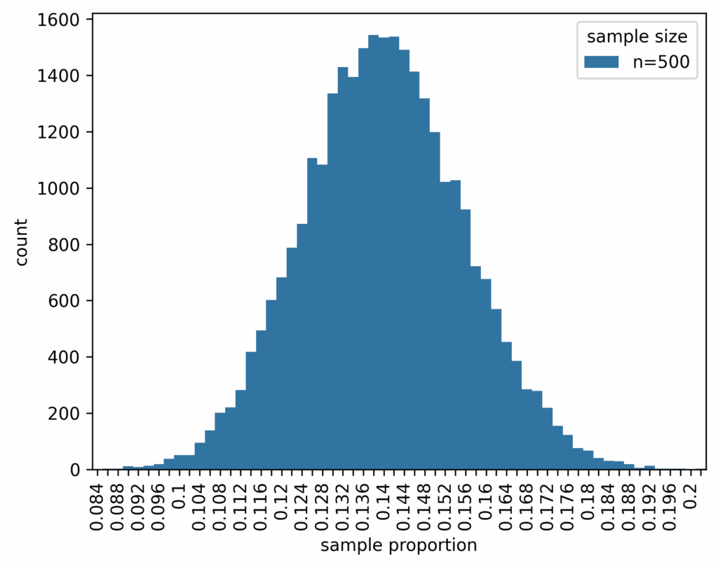
In questions like these it is ofter easier to first start with a god’s-eye-perspective. So we assume that we know already that the difference in conversions of website visit to purchase is 6% between the two variants of the site, 8% of the original version and 14% in the improved version. We have let the A/B test run until 500 samples have been collected for each site, and calculated the conversion proportion. The whole process has been simulated 30.000 times in order to get the sampling distribution. From article 2 we know that with a true proportion of 8% a sample of size 500 will be subject to a distribution that looks like this:

And for the second version of the site it will look like this:
Showing both sampling distributions in one plot, we see that they are clearly different. However, they also overlap:
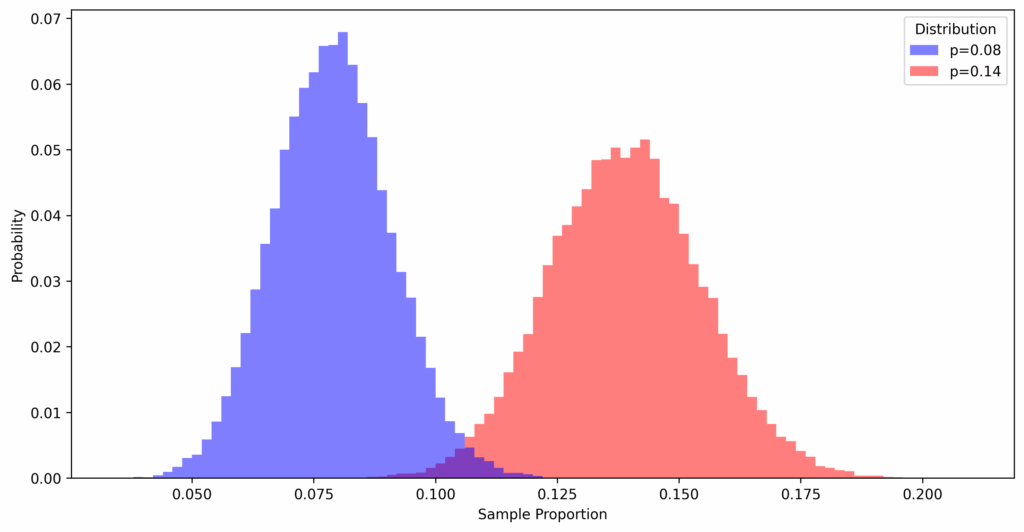
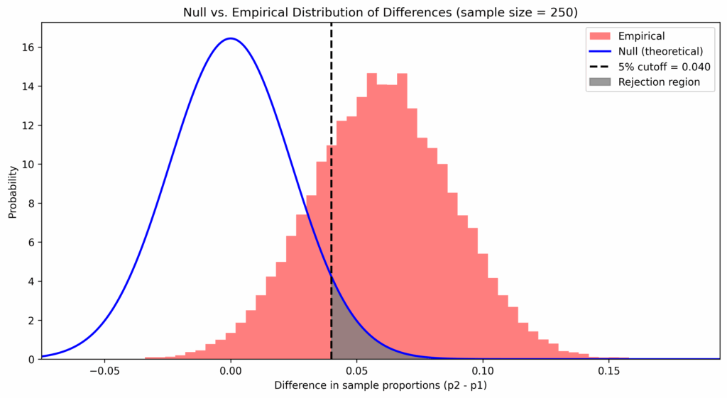
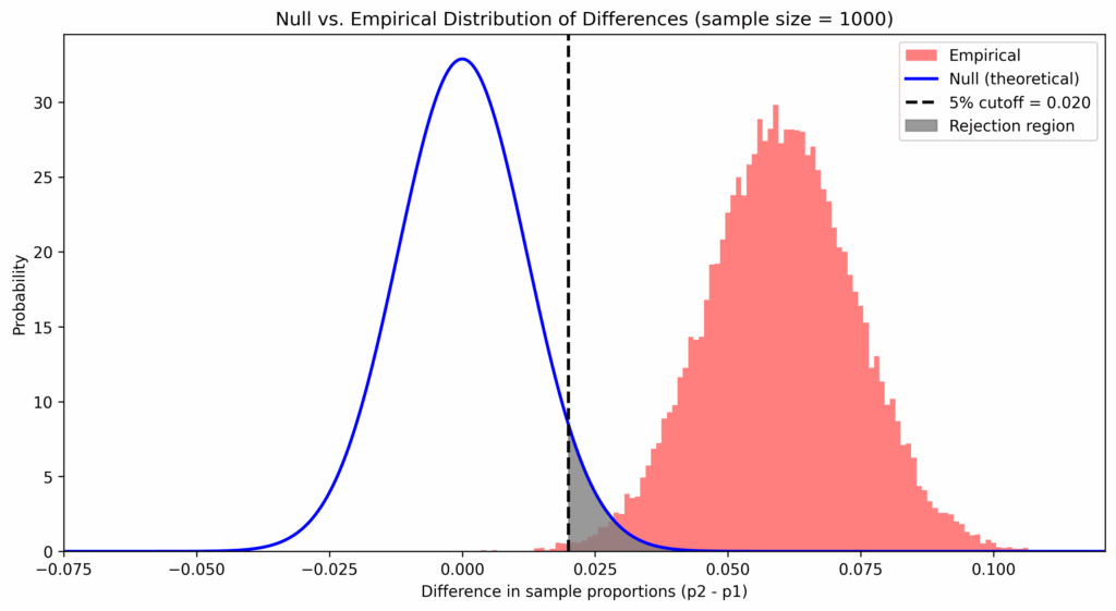
So if we are unlucky and get a sample proportion that lies far to the right of the sampling distribution for the old version and a proportion that lies far to the left for the improved version, someone looking at the sampling results might doubt that there is a genuine difference between the two versions of the website. To determine the question, the following decision rule has become the standard: take the difference of the proportions (improved minus old version) and only accept a value as a genuine improvement if the value is beyond a cutoff value. That cutoff value marks the range of values that can be considered as too extreme, and therefore too improbable, to accept the “null-hypothesis” that there should be no genuine difference between the two versions, and that the extreme value should be merely of product of chance. Seeing the extreme value beyond the cutoff-point, we are rather inclined to believe that another assumption is true, the assumption that the difference is in fact genuine and that that difference has produced the results of the sampling. This is shown in the plot below, where the sampling distribution based on the actual differences from the simulation is shown besides the distribution for the null-hypothesis of “no difference between the two variants”:

Remark that the null-hypothesis is a purely theoretical distribution which we use in the decision rule. There are two aspects of this rule. The first is the cutoff value, this helps us to reject the null-hypothesis. If set too small, we would accept too often measured differences that are merely due to chance. But if we are too cautious and set it too big, we never accept genuine differences because we could always explain the measured results with chance. So how performant the test is in capturing the case of geniune differences, corresponds to how much area under curve of the graph is captured across the range of x’s that are greater than the cutoff value, because it is for exactly those values for which we reject the null hypothesis.
An increase in the level of significance alpha shifts the cutoff value to the right – we are more cautious in ruling out a measured difference merely due to chance. But the downside is we reduce the sensitivity of the test, its capacity to detect geniune differences:

The cutoff-values that need to strike a balance between rejecting too often (type-I-error) and rejecting to little (type-II-error) isn’t the only degree of freedom we have in A/B tests. The sample size is another important factor, as can be seen when their values are to 250 and 1000 respectively. The greater the sample size, the smaller the variation in the sampling distribution, which increases the sensitivity of the test:
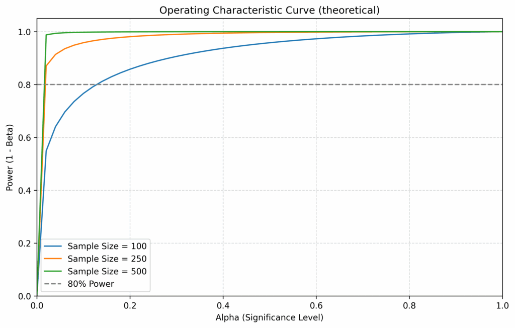
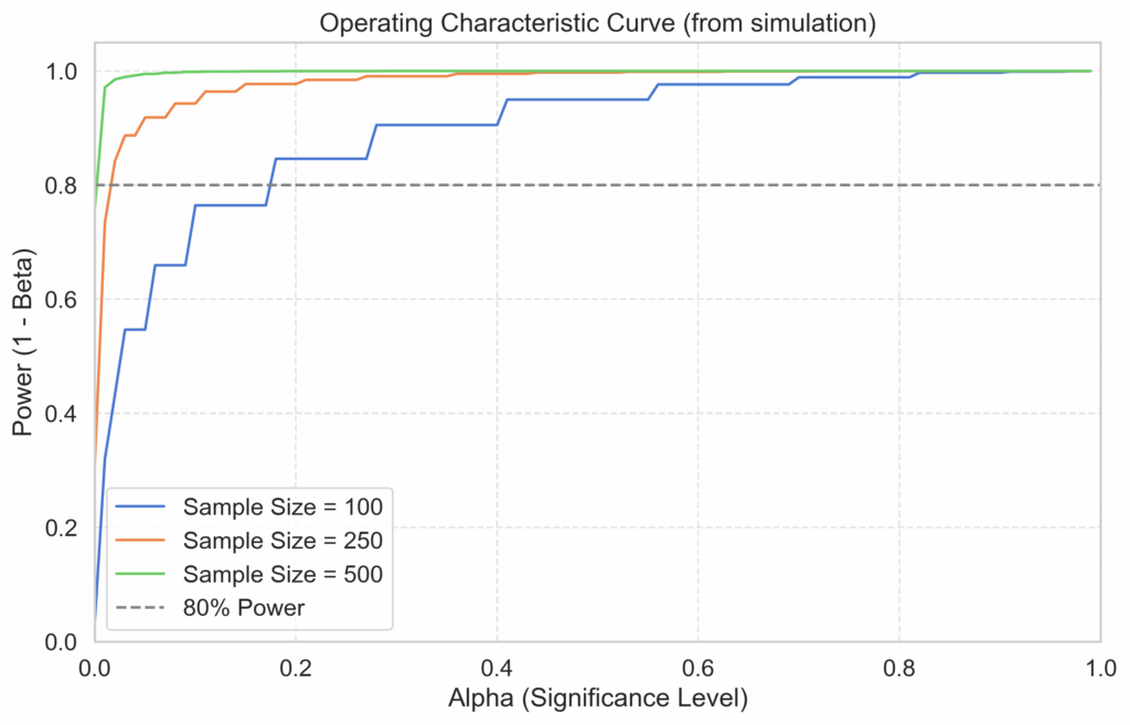
The relationships between the sensivitiy (or power) of the test, the level of significance alpha and the sample sizes can be visualized using the operating characteristic curve. The more we increase the level of significance, the more we are willing to reject the null. Rejecting the null means accepting the alternative explanation of the difference between the proportions of the two compared groups. When the alternative explanation is the genuine difference of 6%, as in the considered example, the power of the test (the capacity of detecting cases of genuine differences) goes up. The happens all the faster if we increase the sample sizes, as with higher numbers the difference in the proportions stands out more and more clearly:
Dropping the god’s eye perspective, the question is not what the true positives and false positives rates are in reality. That’s because we do not know the “true” and “false” cases. We only have the result of our A/B test. Given only that, the questions of relevance are: what is the most likely value of the uplift and what is it error margin? And, more conservatively, what is the minimal reliable value of the uplift, given the fixed value for the certainty of the test?
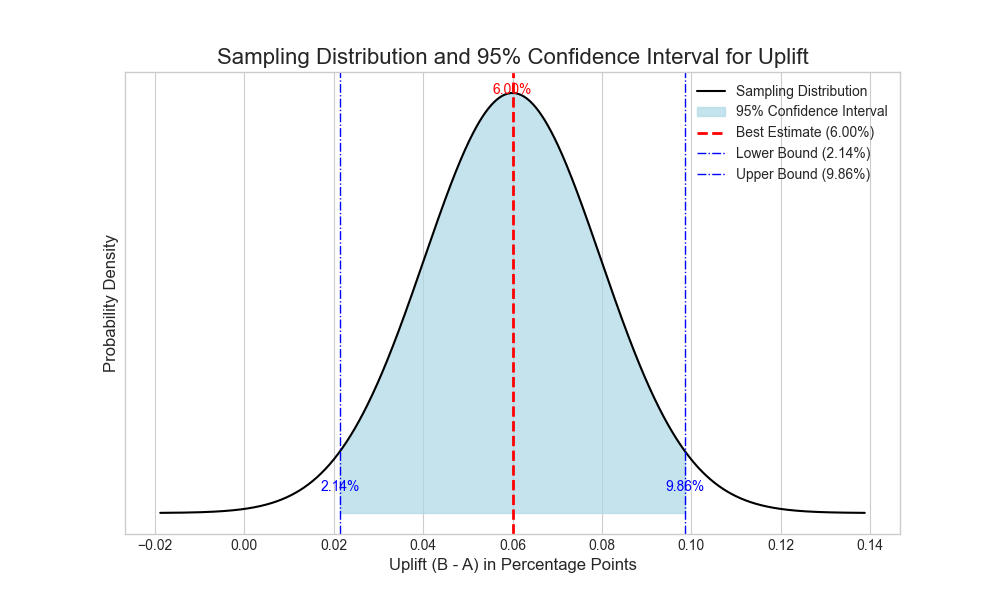
Given the outcome of the one-time sampling of 500 for each of two groups, which resulted in a difference of 0.06, the most likely value for the uplift is, of course, 0.06. But due to the variance of the sampling distribution of differences of proportions, there is an error margin around that value. After a calculation which equals the one made for calculating the cut-off values for rejecting hypotheses, we get 2.14% and 9.86% as the lower and upper limits of the confidence interval around 6% for the uplift. So given the sampling we made this would be the range in which the true uplift lies:
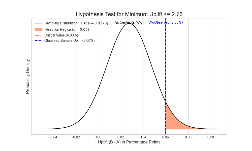
If we instead ask the question, what the minimum positive uplift is in switching from version A to B of the website, the value is even a bit higher, lying at 2.76%. That is because the calculated two-tailed confidence interval, when asking for the most likely value, does not take into account the 2.5% of the probability at the right end of the tail, which stands for extreme positive values in the uplift. Asking for the minimum uplift, we do take that end of the tail into account, so that its 2.5% end up as part of the left end of the tail:
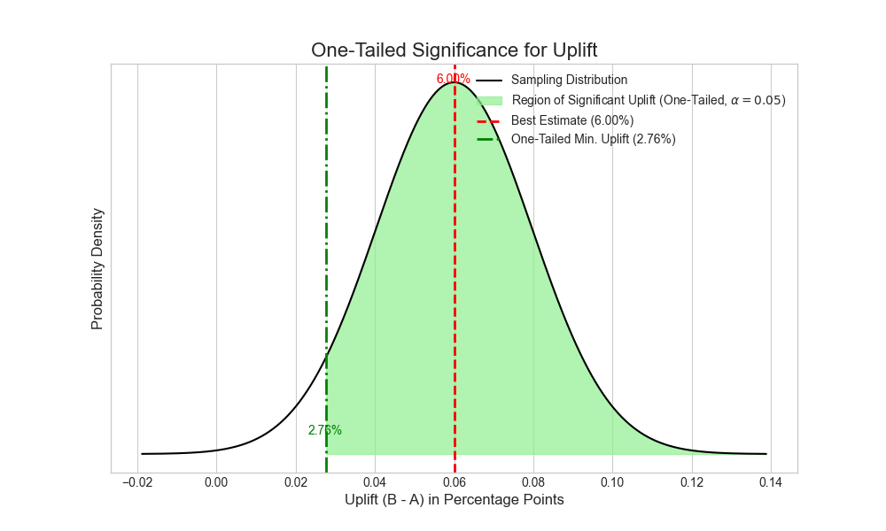
In terms of the null-hypothesis and the alternative hypothesis, this means that we would reject the null-hypothesis that the true uplift is smaller than 2.76%. Why are those two things equivalent? Generally, when we take a sample that yields a proportion (or a mean for that matter) of x, and calculate a value of x_min for the left boundary of the confidence interval for the true proportion, then that is the same as formulating that the hypothesis of the true proportion is x_min, and rejecting that hypothesis on the basis of a sampling result with value x. Both distributions, the one around the sampling result, in order to get the confidence interval, and the one around the supposed true value under the hypothesis, are the same normal distributions, and the difference between the mode and the cutoff-value is also in both cases (x – x_min):