We are victims of the predicament called the fundamental problem of causation because causation is intrinsically counterfactual and its exact quantification would require the observation of the effects of both a causal antecedent and its negation at the same time, which is impossible. We cannot even do the next best thing: build causal models by laying our hands on all manipulable possible causes to our desired effects and measure the actual values of both of them, while also observing all other circumstances outside of our control, but likewise with a bearing on our effects. This is practically not possible. Often we will have to resort to interpreting given data that was measured when we were not around. And data that was probably captured not even in an experimental setup at all. To extract the true causality in such kind of data is step two.
Step one is, of course, to apply classical statistics first, which we will use as a tool throughout and therefore briefly recapitulate here.
The bricks and mortar of our statistical models are the variables and the functions that connect them. The variables can represent either discrete or continuous data. Continuous data can be discretized, but not vice versa. The result of discretization of continuous data is grouped or binned data, which can come in different variants. E.g., the bins containing the instances can be fixed such as to have equal frequencies of those instances, or they can have equal bin widths. The latter case is also called interval data. The least information is carried by data that has been turned into ordinal form, which only preserves the natural order between two instances of the original, continuous form.
All such forms of discretization are to be sharply distinguished from nominal categorical data, which are also discrete, but which do not have a natural order with respect to a second variable.
Next to simplifying statistical models (discrete values might be sufficiently informative), getting the frequencies of the values of the continuous variable can be a reason for discretizing it. Employing probability distribution functions can be a solution, too, but if we do not know that function and only have a sample of values, then binning them to get the frequencies can always be easily done.
More profoundly, the difference between probability distributions and frequencies of a set of measured values consists in that the probability distribution is often an abstract structure that causes the concrete sample taken. E.g., the decisions to make a purchase made by a part of a daily cohort of customers of your web shop can be said to have been produced by the abstract conversion probabilities considering all possible customers of your website at any time. The rate of success in a series of ten free throws that I have made in a particular basketball game are the embodiments of my general capability, quantified by a probability distribution, of performing them. But in other cases the underlying population of possible values from where we draw a sample can also be as concrete as the sample. E.g., when we draw a sample of balls from an urne.
A similar relation of concrete and abstract or factual and potential obtains between the notions of mean and expected value. The mean of a sample can always be calculated based on all concrete values given in the sample. It is a concept from descriptive statistics. The expected value is representative of the population and stands for a value that we would think of as likely to occur when we draw a new sample. It is calculated on the basis of probabilities and is therefore a concept from probability theory.
A confluence of statistics and probability theory is inferential statistics. This is the subfield of statistics that also causal analytics belongs to. We employ it when we use sampling theory in order to predict a statistic of a sample drawn from a known population, or when we use estimation theory to estimate a parameter of the population based on a sample.
A worthy subject to delve into more profoundly is sampling distributions. Around this concept revolves the whole of sampling and estimation theory and with them standard errors, confidence intervalls, hypothesis testing and other concepts of central importance. One can say that sampling distributions are the most decisive concept to grasp if you ever want to get a firm foothold in statistics.
Sampling distributions have something to do with samples, obviously. But with the term we do not mean a description of how the values of an individual sample taken are distributed. An individual sample always has roughly the shape of the population it is taken from, with an increasing resemblance when more and more examples are taken into account. Instead, the sampling distribution refers to how a statistic, like the mean, is distributed when calculated over a collection of different samples. Why we want to look at different samples in the first place becomes clear when we look at the different examples with sampling.
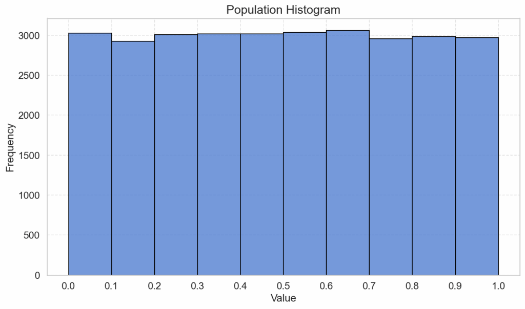
Shown below are the frequencies of values for a population of 30.000 instances of continuous, uniformly distributed numbers from the range of 0 to 1. In order to get frequency plots (histograms), we need to bin those numbers, and for this we use equal bin widths, which gives us the following interval data:
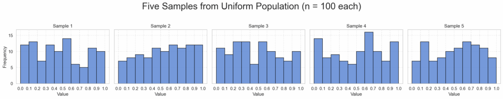
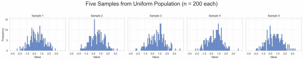
Next, we draw a couple of samples of size 100 and plot them, using the same bins as for the population plot:
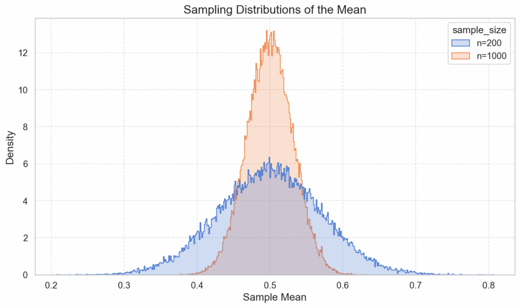
And finally, we plot the “sampling distribution of the mean”, based on 50.000 drawings of samples of size 200 and of size 1000. For each sample, we calculate the mean individually, and count how many times a mean falls into its respective bin, so that we can again plot those occurrences as frequency plots. (In order to get a better comparability between the two curves we use the density plot variant)
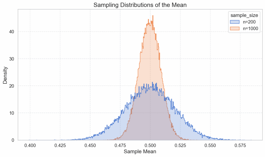
The interesting piece to note is that, while the individual samples’ histograms roughly resemble the uniform distribution of the population, this does not hold true for the sampling distribution of the means taken from the individual samples. This distribution approximates a normal distribution, with a standard deviation that shrinks with the square root.
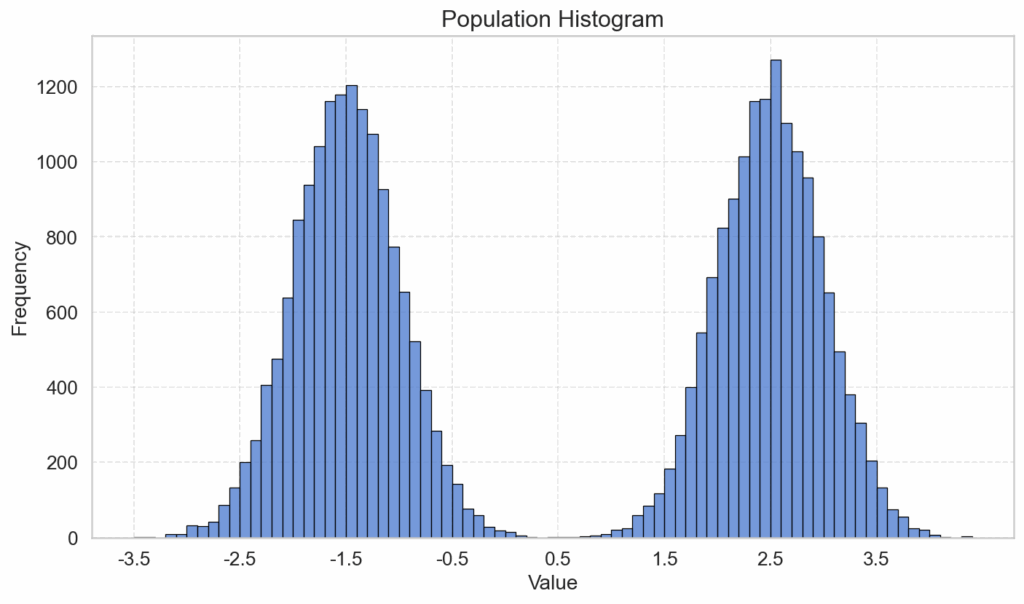
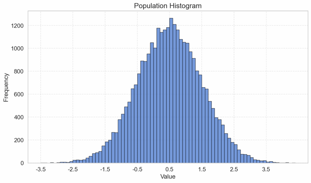
The same pattern emerges for another example with a bimodal distribution, which has been created by having two normal distributions overlap. The two modes are at -1.5 and at 2.5. The population size is 15.000, the sizes of the 5 individual samples plotted are 200, and the data for the plot of the sampling distributions of the mean are the same as in the example before (50.000 drawings of samples of size 200 and 1000):


And, perhaps little surprisingly, the same result with regards to the sampling distribution of the mean can be achieved with a normally distributed population:
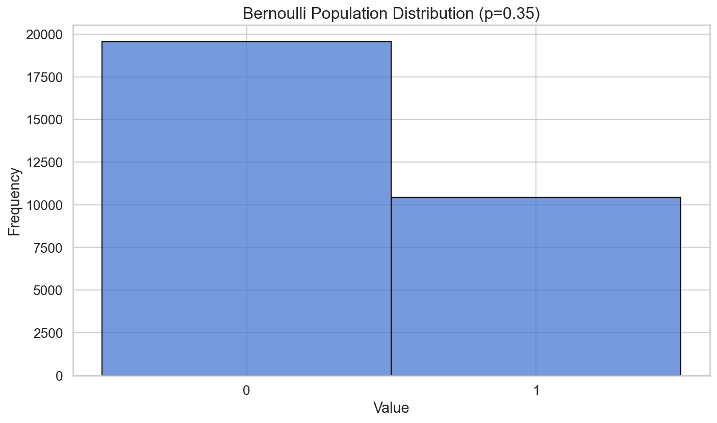
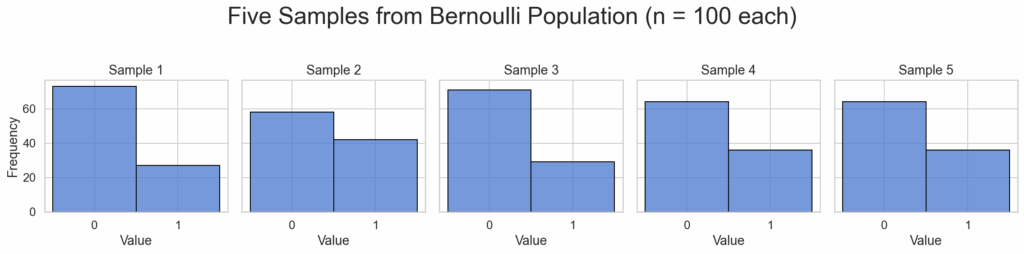
The same works for Bernoulli distributions as well, which only considers proportions of two categories within a population. E.g., whether something is true or false of an individual. Whereas the distribution plot for the population and for the individual samples only consists of two bars, the sampling distribution again increasingly resembles the normal distribution as we increase the sample sizes:

We haven’t yet touched the statistical aspects of the problem of causal inference, because all the above data only involves us as observers, not agents. But this little resumé of classical statistical already reminds us of a pitfall when measuring too little data: the dispersion of our estimates. Parameters of distributions like the mean can only be reliably estimated when lots of data points are taken. Increasing their number is not, however, a remedy against another problem, the conflation of correlation and causation, which is considered in the next article.